Week 5 Bootstrapping, May 10th
This chapter is about the concept of bootstrapping. Like many concepts in this book, bootstrapping is a powerful tool which can be applied to a variety of scenarios, hence it makes sense to gain a firm intuition for the concept first. Fortunately, bootstrapping can be summarized in just two terms: Resampling data in order to investigate the accuracy of estimates (e.g., estimated parameters of a model).
5.1 Gaining an Intuition
But first things first: Why would we want to resample data and what does resampling even mean?
Take a look at the following example: Imagine we have observed a coin which either lands on heads (\(H\)) or tails (\(T\)).
c('T', 'T', 'H', 'H', 'H', 'T', 'H', 'T', 'H', 'H', 'T', 'T')We observed heads 6 out of 12 times. We could conclude that the probability with which the coin lands on heads is \(0.5\). But how confident can we be in making that claim given we have only observed 12 data points? This is where bootstrapping comes into play.
On way of resampling our data through bootstrapping is to simply construct randomized samples of the obtained data with replacement (e.g., draw a random data point n times and return the data point to the pool from which is sampled each time). Usually, the resampled data samples have the same size (i.e. number of data points) like the original sample. Then, for each sample, we compute the frequency with which heads occurs:
dat <- c('T', 'T', 'H', 'H', 'H', 'T', 'H', 'T', 'H', 'H', 'T', 'T')

get_sample <- function(dat)
  return(sample(dat, size=length(dat), replace=TRUE))

get_frequency <- function(dat)
  return(sum(dat=='H')/length(dat))

n_samples <- 10000

samples <- replicate(n_samples, get_sample(dat))

estimates <- apply(samples, 2, get_frequency) # estimate p for all 10000 random samples

quantile(estimates, c(0.025, 0.975)) # 95% confidence interval
## 2.5% 97.5%
## 0.25 0.75You might be asking yourself: “Why is it allowed to re-use the collected data in this way?” - and it is worth considering under which assumptions we resample data during bootstrapping. Typically when we sample data, we presuppose that our sample is an approximation of the sample population. When you estimate results from elections, for example, the population might be all people in Germany that are allowed to vote. Naturally, you can not ask all of these individuals to participate in a survey on their intended voting behavior. Thus, you randomly sample a subset of the population and establish that this sample is representative of the population. Typically, we speak of independent and identically distributed samples. In the example of our coin flips, we might think of independence as the property that the probability of heads does not depend on the outcome of other coin flips and indentically distributed as the property that the probability of a coin landing on heads is constant across all coin flips. Under these properties, we can assume our sample to be an approximation of our population. Therefore, it is reasonable to sample from this approximation during bootstrapping, as we did in the above example with the 12 coin flips. The intuition is that we can expect to draw valid conclusion about our actual population when drawing from an approximation of the actual population, for example when calculating confidence intervals based on bootstrapped estimates. We will elaborate on that idea next.
To recap, bootstrapping follows the following steps:
Collect data
Resample the data to collect a large amount of bootstrap samples
Compute a parameter for each of these samples
Establish a confidence interval (or other metrics) for the resulting parameters
5.2 Bootstrapping in R and the Boot Package
One important distinction to learn in the context of bootstrapping is the difference parametric and non-parametric bootstrapping. The previous example where we sampled the obtained data points with replacement demonstrated non-parametric bootstrapping. In contrast, parametric bootstrapping involves assuming the sample to be following a certain distribution (e.g., binomial), such that we assume certain parameters to determine the probability distribution (hence the name parametric bootstrapping).
To apply this idea to our example with the coin flips, we might sample 1,000 samples of 12 data points from a binomial distribution with \(p=0.5\) (since that is the frequency we estimated in our original sample) and compute an estimate for \(p\) for each of these simulated samples of length 12. Then, we might establish a parametric bootstrap confidence interval for \(p\) based on the 95% least extreme estimations of \(p\). It’s best to visualize the process in R and follow along with the code in your R console:
original_sample <- c('T', 'T', 'H', 'H', 'H', 'T', 'H', 'T', 'H', 'H', 'T', 'T')

initial_estimation_p <- sum(original_sample=='H')/length(original_sample)

n_samples <- 10000

# assuming a binomial distribution with an estimated p, sample n samples with length 12
samples <- replicate(n_samples, rbinom(12, 1, initial_estimation_p))

p_estimates <- apply(samples, 2, mean) # estimate p for all 10000 random samples

quantile(p_estimates, c(0.025, 0.975)) # 95% confidence interval
## 2.5% 97.5%
## 0.25 0.75hist(p_estimates) # plot the distribution of the simulated estimates of p
abline(v=quantile(p_estimates, c(0.025, 0.975)), col='red') # draw 95% confidence interval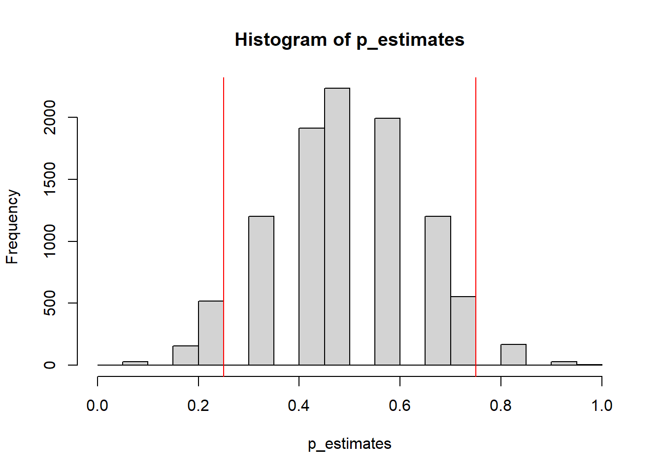
As you can see, the confidence interval we estimated for the parameter \(p\) is quite large, which showcases how 12 data points are not really a good sample size to make accurate inferences about \(p\).
With more advanced models, bootstrapping might not be as simple
as sampling from a binomial distribution. Luckily, there is a very recent (May 2021)
R-package called {boot} which can perform both parametric and non-parametric
bootstrapping. The package might appear
overly complicated at first and one needs to take some time to get acquainted
with its syntax, but the package is very flexible and helpful once mastered.
As will be demonstrated next, the functions of the package need to be instructed (a) which
parameter (e.g., \(\beta\) in a linear regression) to sample and (b) how
to resample the data (e.g., through randomizing rows of a data frame).
Imagine we have a simple linear regression which tries to predict the number of miles per gallon of cars through the number of cylinders of cars. We want to construct a bootstrap confidence interval for the parameter \(\beta\).
\[y = \alpha + \beta x + \epsilon\]
We can take the data set “mtcars”, which is available in R by default, and estimate the parameter \(\beta\) to be \(-2.876\).
lm(mpg ~ cyl, mtcars)##
## Call:
## lm(formula = mpg ~ cyl, data = mtcars)
##
## Coefficients:
## (Intercept) cyl
## 37.885 -2.876But how accurate is this estimation? In order to obtain a bootstrap confidence
interval for \(\beta\), we can
write a function which instructs the package {boot} to fit a linear regression
on randomly sampled rows of “mtcars” and return an estimate for \(\beta\), which
can be obtained through m$coefficients[2] (accessing the model object).
Then, we specify the number of bootstrap samples called R and apply the function
boot() from the R-package which takes the original data,
the instruction function described before, and the number of replications R
as arguments. Saving the return value of this function into an object,
we can easily obtain confidence intervals and a nice density plot for the sampled
\(\beta\) estimators, including a quantile-plot to check normality assumptions of
the model, through the functions boot.ci() and plot(). The result looks like this:
get_beta <- function(dat, index) { # function *must* take at least two arguments
  dat <- dat[index,] # this is where the boot function resamples automatically!
  m <- lm(mpg ~ cyl, dat)
  return(
    as.numeric(
      m$coefficients[2] # return beta estimate
    )
  )
}

result <- boot::boot(data=mtcars, statistic=get_beta, R=1000)

suppressWarnings(boot::boot.ci(result)) # just a demonstration, ignore warnings
## BOOTSTRAP CONFIDENCE INTERVAL CALCULATIONS
## Based on 1000 bootstrap replicates
##
## CALL :
## boot::boot.ci(boot.out = result)
##
## Intervals :
## Level Normal Basic
## 95% (-3.609, -2.159 ) (-3.617, -2.143 )
##
## Level Percentile BCa
## 95% (-3.608, -2.134 ) (-3.657, -2.171 )
## Calculations and Intervals on Original Scaleplot(result)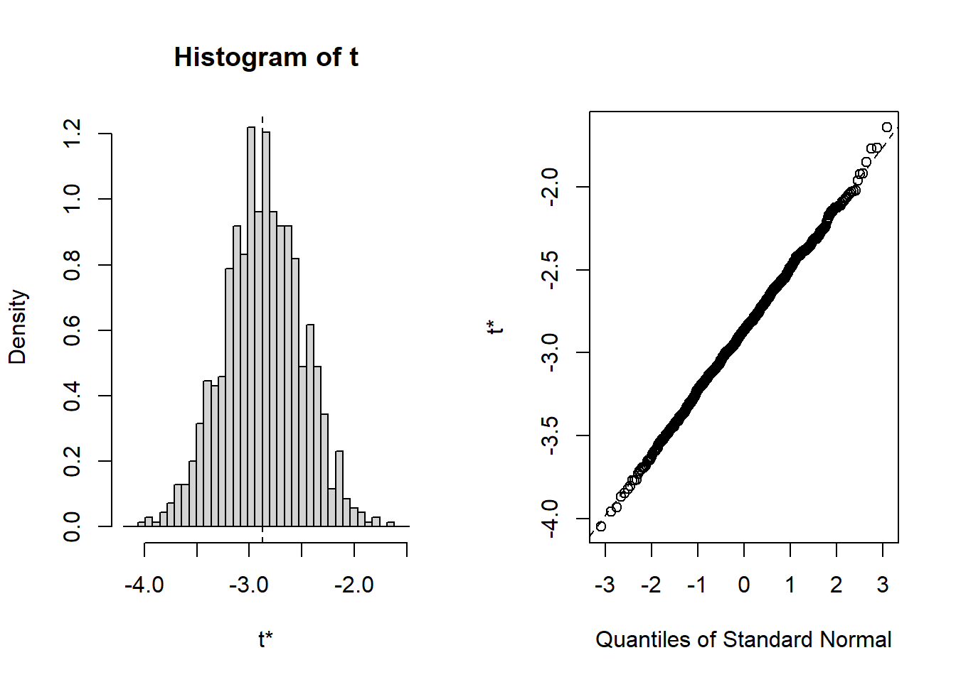
Quite neat, isn’t it? While it takes some time to figure out how to write
the instruction function parsed to the argument “statistic” in the function boot(),
the package {boot} is very much worth learning as it might dominate
bootstrapping with R in the future because of its broad applicability.
Closing remarks: Bootstrapping is a great tool to figure out the accuracy of your sample estimates. Through treating your sample as an approximation of the population under strict sampling assumptions, we can get more information out of our data than we might otherwise think. Given the difficulty of collecting data across many domains, bootstrapping and resampling are thus important concepts to master.