Week 2 Maximum Likelihood I
The maximum likelihood method is essential for estimating and testing parameters across a multitude of models.
Generally, maximum likelihood estimators aim at finding parameters such that the probability of the data given the model parameters is maximized for a pre-defined set of parameters (for example a linear regression model with a slope and an intercept).
In other words, even if we do not exactly know the parameters of a model when we observe data, we can tell what parameters are more likely than others given the data we observed.
2.1 Understanding ML
There are three steps needed to perform maximum likelihood estimation:
Observe data
Calculate the probability of the data given a range of parameter values of the specified model
Set the model parameters of a model such that the likelihood of the data given the model is maximized
Observe data
Imagine you would like to know the probability that it rains on Sundays in London. You could express that probability as the parameter p in a Binomial distribution in which the probability P(X=k) for k successes in n observations with success-probability p is given by:
\[P(X=k) = {n \choose k} \cdot p^k \cdot (1-p)^{n-k}\]
You observe the weather on 2 out of 5 Sundays in London and would like an accurate estimation of p. We obtain
\[P(X=2) = {5 \choose 2} \cdot p^2 \cdot (1-p)^{5-2}\]
Which we can simplify to
\[P(X=2) = 10 \cdot p^2 \cdot (1-p)^{3}\]
Calculate the probability of the results given a range of parameter values of the specified model
Now, let’s imagine we calculate this expression for all possible values of p, which might be any real number in the interval [0, 1]. This means that we calculate what the probability that we observed 2 out of 5 rainy Sundays in London is given different values of p. Then, we take the value of p that maximizes this likelihood in order to obtain our maximum-likelihood estimator.
curve(10*p^2*(1-p)^3, xname="p", from=0, to=1, ylab="L(p)")
abline(v=2/5)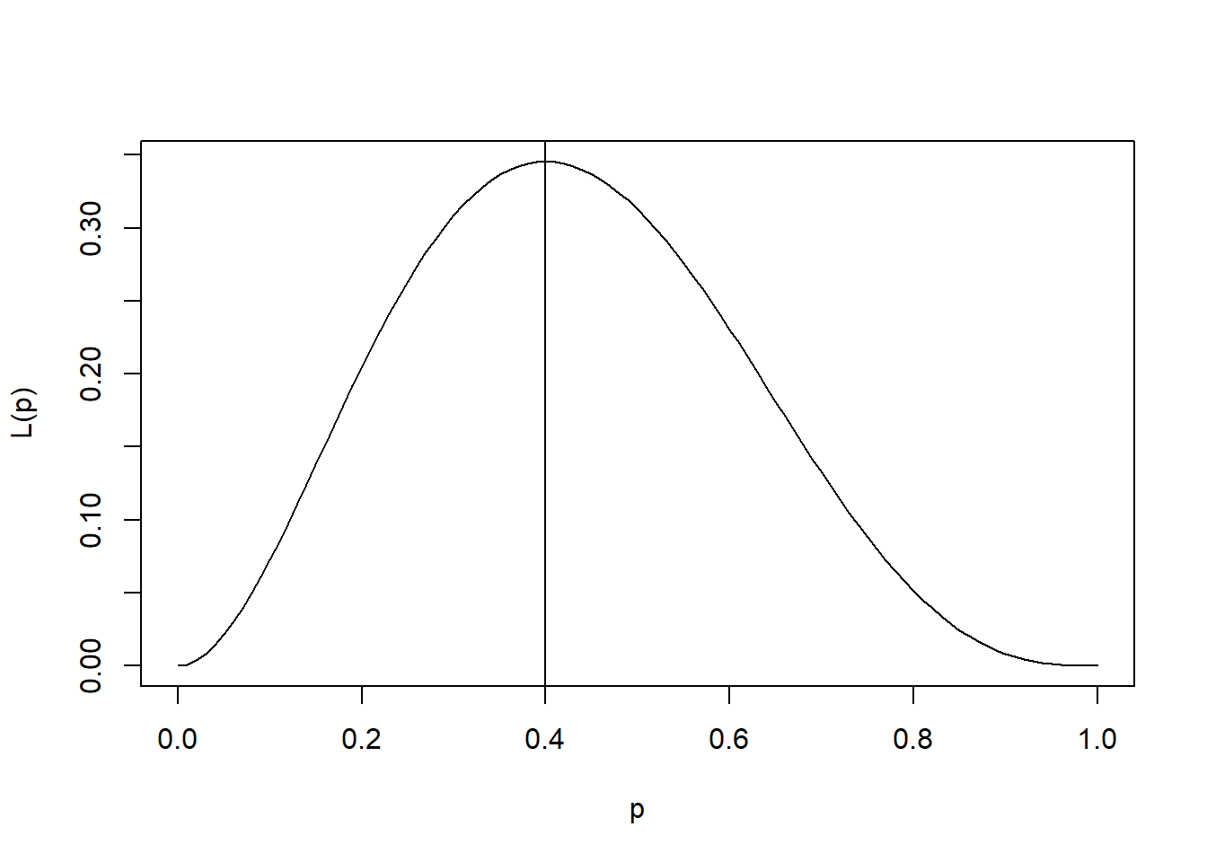
Set the model parameters of a model such that the likelihood of the data given the model is maximized
In this case, the “best” p, that most likely generated the data (2 out of 5 rainy Sundays in London) is 0.4. This quantity also happens to be 2/5 or k/n. We can show that k/n is the optimal solution, or the maximum-likelihood estimator, for any sample following a binomial distribution
2.2 Deriving ML Estimates
An abstract example
Imagine we have two models predicting how likely a coin shows either heads or tails:
| Model | P(heads) | P(tails) |
|---|---|---|
| Model 1 | 0.5 | 0.5 |
| Model 2 | 0.6 | 0.4 |
Model 2 states that the coin is a bit more biased towards heads.
Now we obtain the following data for ten coin flips:
H, H, T, T, H, T, H, T, T, TWe obtained 4 times heads and 6 times tails. Which model does the data most likely come from? Let’s define k as the number of heads in n coin flips with probability p of obtaining heads, which Model 1 sets as 0.5 and Model 2 sets as 0.6. We obtain
Model 1:
\[P(X=4) = {10 \choose 4} \cdot 0.5^4 \cdot 0.5^6 = 0.2050781\]
Model 2:
\[P(X=4) = {10 \choose 4} \cdot 0.6^4 \cdot 0.4^6 = 0.1114767\]
So now we can state that Model 1 is more likely to have generated the data compared to Model 2. Still, there might be even a better model than Model 1 since the maximum likelihood estimator for P(heads) in this situation would be 4/10 = 0.4 which leads to a likelihood of 0.2508227.
A concrete example
Normally, we start with data rather than complete models, so let’s derive that k/n is the maximum likelihood estimator for p in binomial distribution data.
We have seen that we start with the following equation for obtaining the likelihood of p given the data we observed:
\[\mathcal{L}(p) = {n \choose k} \cdot p^k \cdot (1-p)^{n-k}\]
Now, and this is very important to remember, we want to get the maximum of this function (“the most likely value for any possible value of p”). So we have to apply derivation with respect to the parameter p. At the same time, obtaining the derivative of products is challenging, so we first apply the logarithmic operation to the whole equation in order to obtain sums (which are much easier to work with and do not alter the results of what we are trying to obtain).
\[log(\mathcal{L}(p)) = log {n \choose k} + k(log(p)) + (n-k)log(1-p)\]
If this step was too challenging to grasp, please revisit the rules for applying the logarithmic operation to equations.
In our example above, where we tried to estimate the probability of a Sunday in London being rainy, we obtain the following log-likelihood function:
curve(log(10*p^2*(1-p)^3), xname="p", from=0, to=1, ylab="log(L(p))")
abline(v=2/5)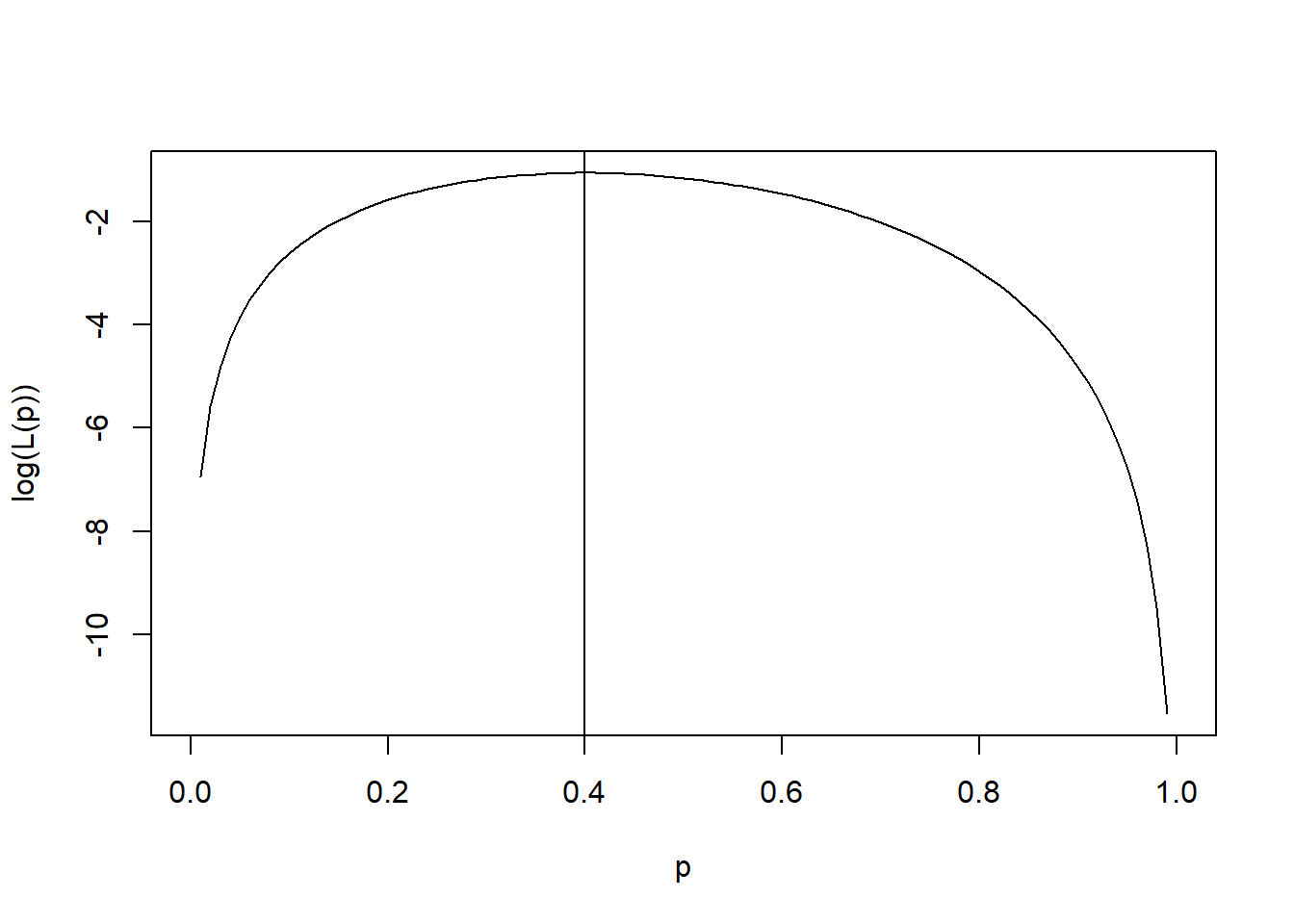
Notice that the value p corresponding to the maximum of the function is still 0.4. Recall that we can derive the argument p which maximizes a function by calculating the first derivative of a function and setting that derivative equal to 0, then solving for p. For \(10 \cdot p^2 \cdot (1-p)^3\) we obtain the log-likelihood \(log(10) + 2log(p) + 3log(1-p)\), for which the derivative with respect to p is \(2/p + (-1) \cdot 3/(1-p) = 0\), since the first component does not contain p and becomes 0, the second component becomes 2 times log(p), since the derivative of \(log(x)\) is \(1 / x\), and the third component needs to be additionally treated with the chain rule [for the inner derivative, (1-p) becomes (-1)]. This equation can then be solved to p = 0.4. If you got stuck in comprehending this derivation, you might revisit some essential rules of how to calculate derivatives here. Plotting this curve, we can also see that the first derivative is 0 for p = 0.4, the maximum-likelihood estimator.
curve(2/p + (-1)*3/(1-p), xname="p", from=0, to=1, ylab="log(L(p)), first derivative")
abline(v=2/5); abline(h=0)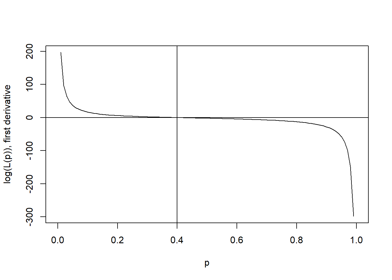
Let’s now apply derivation with respect to p for any set of parameters k, representing the number of successes, and n, representing the number of observations. Remember, we have to set this derivative to 0 and solve it in respect to p in order to obtain the maximum for p, the parameter for which we want to estimate the maximum-likelihood estimator.
For our log-likelihood
\[log {n \choose k} + k(log(p)) + (n-k)log(1-p)\]
the first component again becomes 0, the second component becomes k/p and the third component, again, needs to be treated with the chain rule. We obtain
\[0 = k/p + (-1)(n-k)/(1-p)\]
We multiply this equation with p(1-p) and simplify it in order to obtain:
\[0 = k(1-p)-p(n-k)\] Which is equal to
\[0 = k-pk-pn+pk\] Then
\[0 = k-pn\]
yields our maximum likelihood estimator:
\[p = k/n\]
2.3 More ML Proofs
Let’s derive another maximum likelihood estimator. Again, as you have seen in the example above, we often use the logarithmic operation because sums are much easier to differentiate mathematically than products. At the same time, the logarithmic operation does not alter the maximum of the function (think about the “top of the hill” in the plot above), so there is no harm in working with so-called log-likelihoods.
Poisson Distribution
Given a Poisson distribution (example: how many calls k does a call center receive on day 1, 2, …, i each across n days?) with parameter \(\lambda\) which predicts the probability \(P_\lambda(k)\) for observing k events in the context of count data…
\[P_\lambda(k) = \frac{\lambda^k}{k!}e^{-\lambda}\]
…we can define the likelihood \(\mathcal{L}(\lambda)\) for the parameter \(\lambda\) given a series of n observed event counts \(k_i\) as
\[\mathcal{L}(\lambda | k_1, k_2,...,k_n) = \prod^n_{i=1} \frac{\lambda^{k_i}}{k_i!}e^{-\lambda}\] Applying the logarithmic operation yields
\[log(\mathcal{L}(\lambda | k_1, k_2,...,k_n)) = \sum^n_{i=1}log(\frac{\lambda^{k_i}}{k_i!}e^{-\lambda})\]
Which we can simplify to the following equation, given that \(log(x^k)\) is \(k \cdot log(x)\), \(log(x/y)\) is \(log(x) - log(y)\), and \(log(e^k)\) is \(k\)
\[log(\mathcal{L}(\lambda | k_1, k_2,...,k_n)) = \sum^n_{i=1}[k_i \cdot log(\lambda) - log(k_i!) - \lambda]\] And then simplify to the following equation, given that \((k \cdot x_1 + ... + k \cdot x_i) = k \cdot (x_1 + ... + x_i)\) and \(\sum^n_{i=1}(x) = n \cdot x\)
\[log(\mathcal{L}(\lambda | k_1, k_2,...,k_n)) = log(\lambda) \cdot \sum^n_{i=1}(k_i) - \sum^n_{i=1}log(k_i!) - n\lambda\] Now we can take the derivative of this term with respect to \(\lambda\) as we would like to obtain the maximum likelihood estimator for that parameter and equal the term with 0. Notice how the center part of the equation does not contain \(\lambda\) and thus “drops out” of the equation
\[0 = \frac{1}{\lambda}\sum^n_{i=1}(k_i) - n\] Which can be resolved to
\[\lambda = \frac{1}{n} \sum^n_{i=1}(k_i)\]
So the maximum likelihood estimator for \(\lambda\) is the total number of observed counts across n observations divided by n.
2.4 R Exercises
1. Poisson Distribution
The number of times a police station receives a call in
a given day is conceptualized as being Poisson-distributed.
You observe 6 calls. Plot the likelihood curve of
all possible values of \(\lambda\) in the interval [0, 30]
for this observation.
Click to view the solution
poisson <- function(lambda, k=6, e=exp(1)) {
  return(lambda^k * e^-lambda / factorial(k))
}

curve(poisson(lambda), xname="lambda", from=0, to=30, ylab="L(lambda)")
2. Calculate the probability
Calculate the probability that you observe 5 successes
out of 10 trials in a binomial distribution with
\(p = .4\). Give your answer in \(\%\). Generalize
the solution to any number of successes in the interval
[0, 10].
Click to view the solution
binomial <- function(n=10, k, p=.4) {
  choose(n, k) * p^k * (1-p)^(n-k)
}

result <- binomial(k=5)
round(result, 4)*100
# 20.07%

# General solution for k successes (in %)
round(binomial(k=1:10), 4)*100