Week 6 Model Comparison
In this chapter, we will discuss model complexity, why sometimes a model that may fit the data best is not necessarily the best one to use, and how to find the best model out of a range of candidate model using model comparison methods.
6.1 Model Complexity
When it comes to finding a good model or, more generally, a description of data, we want one that is both accurate and parsimonious. Parsimonious means that we are trying to find a model which is not overly complex and difficult to explain or has other redundant elements. Frequently, this ideal of choosing a parsimonious model is referred to as Ockham’s Razor.
The importance of parsimony is tied to the issue of overfitting, and more generally model complexity. Any dataset we are likely to see is not a perfect reflection of the underlying process we are interested in: It contains noise, and most likely there is variability in data because of stochastic processes. If we try to use a model that captures every single nuance of the data, we are likely to veer into overfitting, or fitting noise instead of the process of interest. In this way, optimizing a straightforward measure of how well our model describes the data, like the RMSE or a MLE, is not enough to be sure we have a good model. Overfitting is generally (but not only) important in the context of model comparison: When we have some candidate models and want to choose the model \(M\) that best captures the essence of the process we are interested in. The rest of this chapter will cover some methods of accomplishing this.
In general, there are several factors that may influence a model’s ability to fit patterns of data (also called model flexibility):
The number of free parameters. This is arguably the most important, and certainly the most heeded factor. Common methods of balancing or evaluating goodness of fit compared to model complexity, like the AIC, take this into account.
The functional form of the model. Even if they have the same number of parameters, an exponential and a power function, for instance, simply have a different functional form.
The parameter space, and bounds placed on it. Constraining the model’s parameters limits its flexibility.
6.2 The Likelihood Ratio Test
In some cases, you may want to compare two nested models, in which one model can be seen as a more general case of the other. This is equivalent to clamping one parameter to a null value, such as 0 or 1 for additive or multiplicative effects. One method to assess whether this parameter actually leads to a better fit for the model, and thus can be seen as capturing some essential part of the processes or mechanisms of interest, is the Likelihood Ratio Test. Let’s assume we are using log-likelihood as a measure of the two models’ goodness-of-fit, calculating the MLE. The deviance is be twice the negative log-likelihood, or \(-2 lnL\). Then, the difference in the deviance between the general and the specific model will be distributed (approximately) according to the chi-square distribution (if the only thing that changes is a parameter allowed to vary freely). \[ -2 log L_{specific} - (- 2 log L_{general}) \approx \chi^2 \] This difference can then be compared to the critical \(\chi^2\) value given \(K\) degrees of freedom, where \(K\) are the extra free parameters gained for the more general model, using a significance level like 0.05.
However, while this test is very simple, it is not without issues. Firstly, it can obviously only be used for nested models. If you want to compare two entirely different models which are not directly related by ‘taking out’ one parameter, you cannot use the Likelihood Ratio Test. But even if you do have nested models, you may not want to use it. The LR test follows the approach of null hypothesis testing, with all the problems that come with it. The validity of this classical approach is a complicated and somewhat thorny topic that is still hotly debated in statistics (if you are interested, there are quite a few papers on this topic, such as this one). Suffice it to say that it can only (attempt to) reject the null hypothesis, and so we cannot find evidence or support for different models.
6.3 The AIC
There are multiple information indexes that represent attempts at quantifying the quality described above (being accurate and parsimonious) for specific models. They typically employ the likelihood of the models given the data (see Chapter 3) and the complexity of the model (most notably represented by the number of parameters of the model). The reason for moving beyond a comparison based on likelihood only is that any model which has all parameters of a less complex model and additional parameters will always fit the data at least equally well. Thus, comparing models only based on likelihood will give complex models an “unfair advantage”. Obtaining indexes that additionally take parsimoniousness into account, we typically choose the model with the lower, hence more favorable, information index.
A very common index that achieves this is the Akaike Information Criterion (AIC), which adds twice the number of parameters to the negative log-likelihood of a model \(M\):
\[AIC(M) = -2 \cdot log L(\hat{\theta}|y,M) + 2k\]
The AIC is derived from the Kullback-Leibler divergence (KL-divergence, also KL-distance). In principle, this is a measure of how much information ist lost trying to approximate one distribution with another, or in this case, one model with another (or reality). It, or more precisely the cross-entropy part of the KL-divergence, is closely related to the expected likelihood of the model given the data. However, the maximized log-likelihood is actually a biased estimate of the KL-divergence, since we use the same data points to get the estimates and calculate this measure. The AIC aims to correct for this bias. It can also be understood as trading off the goodness-of-fit, as examplified by the deviance (the first part of the equation) with the model complexity using a penalty term (the second summand).
An important point to note for using the AIC is that it does not hold up as well for small samples, when there is a large number of parameters given the data points. In such cases, it is better to use the corrected AIC, with \(n\) referring to the number of data points and \(k\) the parameters:
\[AIC_c(M) = -2 \cdot log L(\hat{\theta}|y,M) + 2k * (\frac{n}{n-k-1})\] In general, it is important to note that the AIC values you may get depend on the model and data, and cannot easily be compared across different situations. In fact, what matters is not the actual AIC value but the difference between them for candidate models: a difference of \(\Delta AIC\) of 2 expresses the same strength of evidence for a model compared to another when you have AIC values of 10 and 12 or 1000 and 1002!
6.3.1 A simple example
We’ll go back to our trusty linear regression. This time, we’ll compare two models, one of which is your standard linear regression and one a simpler version that does not include an intercept parameter. Let’s generate some data.
NumberOfSamples <- 100
Slope           <- .8
Intercept       <- .1
stdNoise        <- .5
data <- matrix(0, NumberOfSamples, 2)
set.seed(123)
data[ ,2] <- rnorm(NumberOfSamples)
data[ ,1] <- rnorm(NumberOfSamples) * stdNoise + data[ ,2] * Slope + Intercept
Now, we’ll specify the models and get some parameter estimates for both of them, using the lm function for convenience. Firstly, let’s use a model with both an intercept and a slope parameter.
model_1 = lm(data[,1] ~ data[,2], as.data.frame(data))
model_1$coefficients
## (Intercept) data[, 2]
## 0.04859847 0.77376419And for comparison, a model where the intercept is set to 0 and we only have one free parameter, the slope:
model_2 = lm(data[,1] ~ 0 + data[,2], as.data.frame(data))
model_2$coefficients
## data[, 2]
## 0.7790381Now, we calculate the AICs and look at the difference. For this, we can use the built-in ‘AIC’ function
print(AIC(model_1))## [1] 143.1935print(AIC(model_2))## [1] 142.2014delta_AIC = AIC(model_1) - AIC(model_2)
print(delta_AIC)## [1] 0.9920858As you can see, the difference in AIC is about 0.99, which is not particularly high. Remember that this \(\Delta AIC\) is what you should pay attention to rather than the specific AIC values! We can see that neither model has particularly strong support compared to each other.
6.4 The BIC
Another common measure is the Bayesian Information Criterion (BIC), which additionally takes into account the number of data points \(n\) through which evidence has been accrued.
\[BIC(M) = - 2 \cdot log L(\hat{\theta}|y,M) + k * log(n)\]
The BIC is based on Bayesian principles. Specifically, it is derived using the Laplace approximation for marginal likelihood. As you might notice, however, despite having ‘Bayesian’ in the name, there’s no reference to the prior distribution, which you would normally expect to get the posterior distribution in Bayesian updating (we’ll learn more about that in a later session). In fact, it does use the so-called unit information prior, which is implicitly assumed in the BIC by the way it is derived. Arguably, this fails to take advantage of a strength of the Bayesian approach, being able to quantify and use your prior knowledge, but it makes for an easy and simple measure, similar to the AIC.
In comparison, the BIC is often found to be a more conservative estimate than the AIC, which means that model complexity gets punished more severely. For instance, if we go back to nested models and look at a caste with one additional parameter, the maximum difference in AIC for a specific versus general model can be 2 at most (since \(k\) = 1). This is not the case for the BIC, where with large \(n\) we can find much stronger support for the simple model. However, it must be kept in mind that AIC and BIC are taken from different frameworks, and it is hard to directly compare them. They do not always agree, and which one to use can be is not a question with a straightforward answer. Either way, however, note that both AIC and BIC only take the number of parameters of the model into account when it comes to model complexity, not its functional form.
6.4.1 Example
Let’s continue with the same example and see if using the BIC would differ from the AIC. As a reminder, these are the data and the models we used:
# simulated data
NumberOfSamples <- 100
Slope           <- .8
Intercept       <- .1
stdNoise        <- .5
data <- matrix(0, NumberOfSamples, 2)
set.seed(123)
data[ ,2] <- rnorm(NumberOfSamples)
data[ ,1] <- rnorm(NumberOfSamples) * stdNoise + data[ ,2] * Slope + Intercept

# example models
model_1 = lm(data[,1] ~ data[,2], as.data.frame(data))
model_2 = lm(data[,1] ~ 0 + data[,2], as.data.frame(data))
We can calculate the BIC simply as well, for the same data and using the same models as above:
print(BIC(model_1))## [1] 151.009print(BIC(model_2))## [1] 147.4117delta_BIC = BIC(model_1) - BIC(model_2)
print(delta_BIC)## [1] 3.597256Here, our \(\Delta BIC\) is about 3.6. This is considerably larger than using the AIC, so we would conclude that this measure gives stronger support to the first model.
6.5 Bonus: Monte Carlo and Minimum Description Length
There are ways to take the functional form of a model into account, not just its number of parameters like AIC and BIC, although these measures tend to be harder to calculate. Here, we will touch on Monte Carlo methods and the concept of Minimum Description Length.
6.5.1 Monte Carlo Methods
Monte Carlo methods refer to approximations through simulation. Specifically, they entail
drawing a large amount of data points from the same distribution
estimating some kind of index or property of that distribution
Why would we want to do that? The short answer is: Simulating is sometimes easier than solving mathematical equations. The long answer: Monte Carlo simulations work across a large variety of contexts, as will be demonstrated in this section and beyond!
The intuition behind Monte Carlo simulations is that if we sample from a given distribution often enough, we will obtain a sufficiently approximate estimate of the index / property we are looking for. This is due to the law of large numbers, which states that the average of the data points from a large number of trials converges to an expected or theoretical value and gets closer to that expected or theoretical value the more data points are sampled.
Still too abstract? Here goes a simple example:
Imagine we have a normal distribution \(X \sim \mathcal{N}(\mu, \sigma^2)\). Let’s also imagine that \(\mu\) is actually 0. Now, we can sample data points from that normal distribution and estimate \(\mu\) through calculating the mean of the sampled data points. The law of large numbers states that our approximation of \(\mu\) will tend to be closer to the actual value, which in this case is 0, the more data points we sample.
Here is some R code which demonstrates this:
set.seed(1)

the_sampled_data_points <- rnorm(n=5)
our_estimation <- mean(the_sampled_data_points)
our_estimation # not really close...
## [1] 0.1292699the_sampled_data_points <- rnorm(n=50)
our_estimation <- mean(the_sampled_data_points)
our_estimation # getting there...## [1] 0.09613849the_sampled_data_points <- rnorm(n=50000)
our_estimation <- mean(the_sampled_data_points)
our_estimation # close enough!## [1] -0.002728035You could consider the above example to be a rudimentary Monte Carlo simulation. But there is much more to simulate! Through Monte Carlo simulations, we might simulate areas, distributions, model parameters, among others. One common application is the approximation of integrals, as we will discuss next.
6.5.2 Exemplary MC Integrations
Imagine we would like to solve the following integral:
\[\int_0^3 x^2 \,dx\]
Not much of an intimidating task, is it? This is because there is a closed solution to solving this integral. In other words: We can apply arithmetic and integration rules to obtain the solution to this integral.
In this case, we get:
\[\int_0^3 x^2 \,dx = \frac{3^3}3+C = 9\]
Let’s actually visualize the area under the curve of \(f(x)=x^2\):
curve(x^2, 0, 3)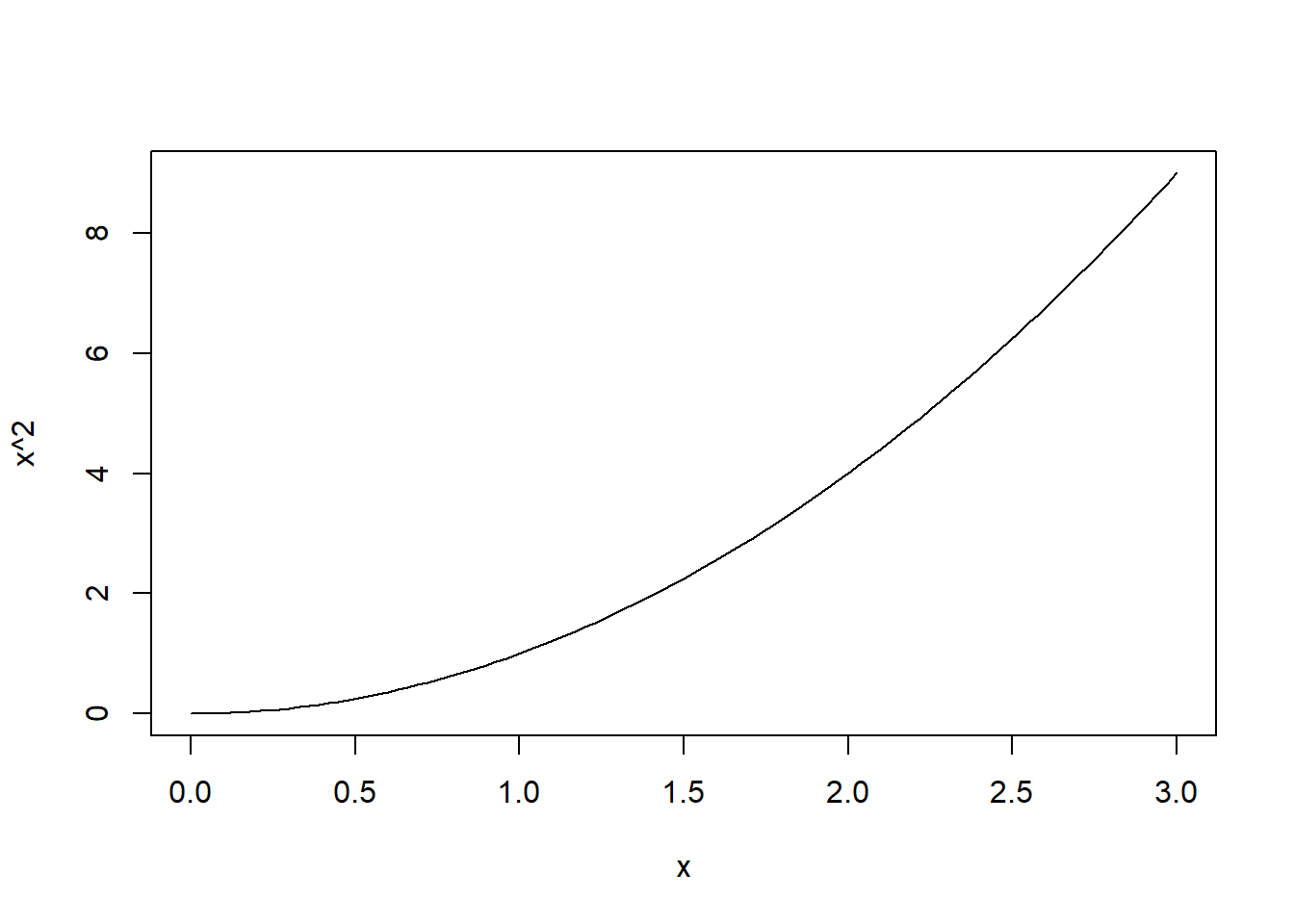
You could conceptualize this graph as a two-dimensional plane made up of \(x\) and \(x^2\) in the interval \([0, 3]\). Notice that this plane establishes a rectangle with an area of \(x*x^2 = 3*3^2 = 27\) square units. Any point within this area is a pair \((x_1, x_2)\) where \(x_1\) is drawn from the a uniform distribution in the interval \([0, 3]\) and \(x_2\) is drawn from a uniform distribution in the interval \([0, 3^2]\). We can then simulate \(N\) tuples \((x_1, x_2)\) and observe the ratio with which \(x_2 < x_1^2\) holds. This ratio represents the time a random data point \((x_1, x_2)\) is under the curve \(f(x)=x^2\) in the two-dimensional plane we established. We can then obtain an approximation of the actual area under the curve \(f(x)=x^2\) in the interval \([0, 3]\) if we multiply this ratio with the total number of square units, which is 27, as shown previously. If we did everything correctly, this estimation should be approximating 9, the correct solution to the integral. Let’s try this in R!
set.seed(121)
area_of_2d_plane <- 3*9
n_simulations <- 100000
x1 <- runif(n=n_simulations, min=0, max=3)
x2 <- runif(n=n_simulations, min=0, max=9)
ratio <- sum(x2 < x1^2) / n_simulations
ratio*area_of_2d_plane # should be ~ 9
## [1] 9.00612plot(x1, x2, pch=".", col=ifelse(x2 < x1^2, "red", "grey"),
main="MC Integral Approximation")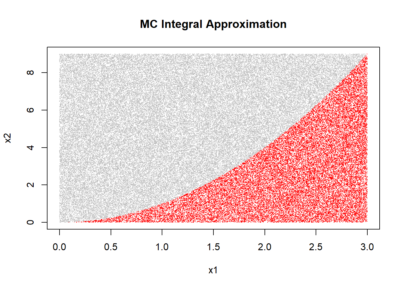
Now, one can observe how the randomly sampled points \((x_1, x_2)\) for which \(x_2 < x_1^2\) holds are indeed those under the curve \(f(x)=x^2\).
Such an approximation is an example of a Monte Carlo simulation. In cases where there is no closed solution (or a computationally very resource-intense solution) to an integral, we can use Monte Carlo simulation to still obtain an approximation of that integral. This method can be generalized to higher dimensions (i.e., multivariate functions) and is often used to approximate a-posteriori distributions in Bayesian statistics (referred to as Markov Chain Monte Carlo methods).
6.5.3 Minimum Description Length (MDL)
When trying to understand the concept of minimum description length (or MDL), there are two aspects to consider. First, there is a general intuition behind the idea of the description length of models describing regularities in data. Second, there are mathematical formulas corresponding to indexes of models that help us decide between two models in terms of whose MDL is more favorable.
As mentioned above, we have the goal of finding models that are both accurate and parsimonious.
6.5.3.1 Determinants of Matrices
To calculate the determinant of a \(2\times 2\) matrix \(A = \bigl(\begin{smallmatrix} a&b \\ c&d \end{smallmatrix} \bigr)\), the formula \(det[A] = a * d - b * c\) can be used.
For a \(3\times 3\) it is necessary to consider a checkered pattern of signs:
\[\begin{pmatrix} + & - & + \\ - & + & - \\ + & - & + \end{pmatrix}\] Then, in order to calculate the determinant, a row or column of the matrix has to be selected. It does not matter which row or column is used, but the calculation might be easier depending on the choice. In this example, the first row of the matrix is used:
\[A = \begin{pmatrix} a & b & c \\ d & e & f \\ g & h & i \end{pmatrix} \]
That the first row is used means that each element of the first row, with the corresponding sign at it’s location in the sign matrix above, is multiplied with the determinant of a \(2\times 2\) matrix consisting of the 4 numbers that are not in the same row and column as the element. The results for every element in the selcted row are then added together. The formula will make it easier to understand:
\[det[A] = +a * det[(\begin{smallmatrix} e&f \\ h&i \end{smallmatrix})] -b * det[(\begin{smallmatrix} d&f \\ g&i \end{smallmatrix})] +c * det[(\begin{smallmatrix} d&e \\ g&h \end{smallmatrix})]\]
For bigger matrices, this process can be applied recursively. Once again, a row or column needs to be selected and the checkered sign matrix needs to be extended in the same way.
Exercises
Calculate the determinants of these matrices: \[ A = \begin{pmatrix} 2 & 3 & -0.5 \\ 2 & 5 & -1 \\ 1 & -1.5 & -2 \end{pmatrix} \\ B = \begin{pmatrix} 2 & -2.3 & 1.25 \\ 4 & 5.76 & -0.5 \\ 0 & 7 & 0 \end{pmatrix} \\ C = \begin{pmatrix} 2 & 3.2 & -4 \\ 1 & -2 & -2 \\ -3 & 1 & 6 \end{pmatrix} \\ D = \begin{pmatrix} 1 & 0 & 3 & -2 \\ 2 & -1 & 0 & -1 \\ 0 & 3 & -2 & 1 \\ 4 & 0.5 & 1 & -2 \end{pmatrix} \\ \]Click here to see the solutions
\[ det[A] = -10 \\ det[B] = 42 \\ det[C] = 0\\ det[D] = 10 \]
In Matrix C, columns 1 and 3 are multiples of each other. In this case, the determinant will always be 0.
6.5.3.2 Inverses of Matrices
The inverse \(A^{-1}\) of a \(n\times n\) matrix \(A\) is defined in the following way: \(A * A^{-1} = I_n\) For example:
\[A * A^{-1} = \begin{pmatrix} 1 & 2 \\ 2 & 3 \end{pmatrix} * \begin{pmatrix} -3 & 2 \\ 2 & -1 \end{pmatrix} = \begin{pmatrix} 1 & 0 \\ 0 & 1 \end{pmatrix} = I_2\]
The inverse of a matrix can be calculated in the following way:
Let \(A =\bigl(\begin{smallmatrix} 1&2 \\ 3&4 \end{smallmatrix} \bigr)\). Then, this matrix A is put into a system with the identity matrix of the same size:
\[ \big(\begin{array}{c|c} A & I_2 \end{array}\big) \\ \bigg(\begin{array}{cc|cc} 1 & 2 & 1 & 0\\ 3 & 4 & 0 & 1 \end{array}\bigg)\]
Then, to obtain the inverse, the left side is transformed into \(I_2\) through elementary matrix operations. The matrix on the right side is the inverse:
\[ \big(\begin{array}{c|c} I_2 & A^{-1} \end{array}\big) \\ \bigg(\begin{array}{cc|cc} 1 & 0 & -2 & 1\\ 0 & 1 & 1.5 & -0.5 \end{array}\bigg)\]
The same procedure applies for larger matrices. For \(2 \times 2\) matrices, the following formula applies to directly calculate the inverse:
\[A^{-1} = \frac{1}{det[A]}\begin{pmatrix}d & -b \\ -c & a\end{pmatrix}\]
Note: A square matrix \(A\) is invertible if and only if \(det[A] \neq 0\).
Exercises
Calculate the inverses of these matrices: \[ A = \begin{pmatrix} 1 & 2 \\ 0 & 1 \end{pmatrix} \\ B = \begin{pmatrix} 2 & -1 \\ -4 & 3 \end{pmatrix} \\ C = \begin{pmatrix} 2 & -3 \\ -4 & 6 \end{pmatrix} \\ D = \begin{pmatrix} 1 & 0 & 2 \\ 0 & 1 & 3 \\ 2 & 1 & -1 \end{pmatrix} \\ \]
Click here to see the solutions
\[ A^{-1} = \begin{pmatrix} 1 & -2 \\ 0 & 1 \end{pmatrix} \\ B^{-1} = \begin{pmatrix} 1.5 & 0.5 \\ 2 & 1 \end{pmatrix} \\ det[C] = 0 \implies \text{no inverse}\\ D^{-1} = \begin{pmatrix} 0.5 & -0.25 & 0.25 \\ -0.75 & 0.625 & 0.375 \\ 0.25 & 0.125 & -0.125 \end{pmatrix} \\ \]
6.5.3.3 Aspect 1 - Description Length Intuiton
Imagine we have the following vector:
c(1, 1, 2, 2, 1, 1, 2, 2, 1, 1, 2, 2)## [1] 1 1 2 2 1 1 2 2 1 1 2 2As you can see, there is regularity in this data. You might think of a model (or description) that accurately predicts these data:
Repeat c(1, 1, 2, 2) thrice.
We might also come up with a more algorithmic description:
Start with c(1, 1). For index n, if numbers of indexes n-1 != n-2 then number n-1 is number n. Else change to 2 if number n-1 is 1 and 1 and 1 if number n-1 is 2. Do while the vector has not length 12.
We can implement both descriptions in R:
# A
rep(c(1, 1, 2, 2), 3)
## [1] 1 1 2 2 1 1 2 2 1 1 2 2# B
v <- c(1, 1)
while(length(v) < 12) {
n <- length(v)
if (v[n] != v[n-1])
v <- c(v, v[n])
else
if (v[n] == 1)
v <- c(v, 2)
else
v <- c(v, 1)
}
v## [1] 1 1 2 2 1 1 2 2 1 1 2 2As you can see, while both programs are equally accurate, the first one is more parsimonious (it literally has a shorter “description length”). It, therefore, has a more favorable MDL.
6.5.3.4 Aspect 2 - Description Length Indexes
The book Computational Modeling of Cognition and Behavior by Farrell and Lewandowsky provides us with a more adventurous formula which extends the logic of the BIC through additionally considering the determinant of the observed Fisher information matrix:
\[MDL(M) = -log L(\hat{\theta}|y,M)+\frac{K}{2}log(\frac{N}{2\pi})+log\int d\theta\sqrt{det[I(\theta)]}\] In the next chapter, you will be able to find more information on the Fisher information matrix. In the meantime, in case you are not familiar with the concept of matrix determinants, here is a short article which gives an intuition for the geometric interpretation of determinants based on matrix multiplication.
In the MDL formula, the first term refers to the goodness of fit of the model, just like in the AIC and BIC. Accordingly, the second and third term punish model complexity. However, these terms are more complex, thus it is useful to look at what they mean in order to get an intuition of what MDL does. Most of the following explanations are taken from this paper.
In general, a statistical model is a collection of probability distributions dependent on the parameters \(\theta\). The idea of MDL is to describe model complexity by counting the number of distributions that a model can generate. The more distributions a model can generate, the more complex it is. However, with continuous parameters, there always are uncountably infinite distributions. So, a small trick is needed to actually be able to count them. As an example, let us consider two normal distributions that only differ in their mean. If the difference between the means is small enough, even with a large number of values drawn from the two distributions, we would not be able to distinguish them. Then, we can consider these distributions as indistinguishable and thus count them as one. So we consider all indistinguishable distributions with approximately the same mean as members of the same region and count the regions. We now have countably(!) infinite different distribution regions. To account for the continuous parameters, it is necessary to take the limit of samples drawn from the distributions. With the limit of samples going to infinity, the regions of indistinguishable distributions will shrink. In the formula, this number of distinguishable distributions is expressed by \(d\theta\sqrt{det[I(\theta)]}\), where \(d\theta\) refers to taking the limit. This then needs to be integrated over the whole parameter manifold: \(V_m = \int d\theta\sqrt{det[I(\theta)]}\). This is called the Riemannian volume, which describes the number of distributions a model can generate.
But why exactly does this formula describe the number of distributions? To get an intuition for that, it is useful to know that the inverse of the fisher information matrix is often used as an approximation of the covariance matrix. So let us first consider the meaning of the determinant of the covariance matrix. The determinant of the covariance matrix is called generalized variance and gives a measure of how dispersed the generated points are (to understand this, it could be useful to go trough a calculation of the generalized variance in the 2d case). But what is the impact of the generalized variance on the number of distinguishable distributions? If the distributions generated by the parameters have high variance, a small change in parameters (i.e. the mean) does not make the distributions as distinguishable as the same change would for distributions with lower variance. Here is a visualization of this:
x <- seq(-2,2,0.01)
mean1 = -0.25
mean2 = 0.25
sd1 = 0.2
sd2 = 2
plot(x, dnorm(x,mean1, sd1), type="l", main="Normal distributions", ylab = "y")
lines(x, dnorm(x,mean2, sd1), col="red")
lines(x, 10*dnorm(x,mean1,sd2), col="black") #factor 10 for better comparison
lines(x, 10*dnorm(x,mean2,sd2), col="red")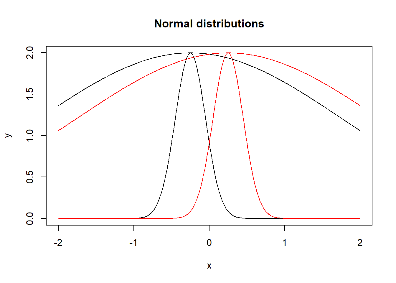
Both black and both red distributions have the same mean with different variances. As you can see, the narrow distributions with \(\sigma = 0.2\) are easily distinguishable whereas the distributions with \(\sigma = 2\) are not. Therefore, in the case of high generalized variance, the regions of indistinguishable distributions are larger and the model can thus generate less distributions, it is less complex. In this case, the determinant of the covariance matrix is large. Because of the relation \(det[A^{-1}] = \frac{1}{det[A]}\) this means that the determinant of the fisher matrix is small. So the MDL is lower for a less complex model, which is what we want.
Additionally to the total number of distributions, MDL also considers the number of distributions that are acceptably close to the true distribution that generated the data. Essentially, this is the Riemannian volume of a small ellipsoid around \(\hat{\theta}\) denoted as \(C_m\).
For a model it is beneficial if the number of generatable distributions acceptably close to the truth is large whereas the total number of distributions is small. This can be achieved by minimizing \(\frac{V_m}{C_m}\) or, as in MDL, the log of this: \[log(\frac{V_m}{C_m}) = \frac{K}{2}log(\frac{N}{2\pi})+log\int d\theta\sqrt{det[I(\theta)]}+log(h(\hat{\theta}))\] The term \(log(h(\hat{\theta}))\) can be neglected as it is a data dependent factor going to 1 for large \(N\).
To sum this up, the MDL punishes model complexity not only in terms of the number of parameters but instead in terms of distributions that a model can generate. Obviously, more parameters can generate more distributions and are thus punished like in the AIC. However, the complexity of two models can vary even with the same number of parameters. This is not taken into account by the AIC. Thus, the MDL uses a more general approach to model ceomplexity.
Since all three formulas will not always lead to the same conclusion when comparing two models, they may not be taken as unmistakable evidence for the superiority of one model over another. Rather, they can give an intuition on which out of two models might be overly complex with respect to the additional likelihood gained through the added model parameters. Remember - any model which has all parameters of a less complex model and additional parameters will always fit the data at least equally well.
Here is an example of comparing two models through the AIC in R.
Can you figure out whether the speed predictor describes a
accurate and parsimonious variable when predicting the variable dist?
m0 <- lm(dist ~ 1, cars)
m1 <- lm(dist ~ speed, cars)
AIC(m0)
AIC(m1)
6.5.3.5 Closing thoughts
MDL is an abstract concept with important methodological implications. Adding MDL to your methodological toolbox will help you evaluating model fit with data you obtained. Specifically, considering both accuracy and parsimoniousness will reduce the probability of choosing a model that is highly fitting with the data but does not generalize well to new data, as happens with overfitting.
6.5.4 R Exercises
Exercise 1:For any normal distribution \(X \sim \mathcal{N}(\mu, \sigma^2)\), simulate the frequency of a data point \(x_i\) being 2 standard deviations below the mean.
Click here to obtain a hint
Sample from a normal distribution through the functionrnorm().
Click here to see a possible solution
n <- 1000000
sum(rnorm(n)<(-2))/nAlready in ancient Greece, mathematicians have been concerned with “squaring the circle”, which means to construct a square such that the area of that square is equal to the area of a given circle. The reason for the difficulty of the task is arguably the irrational constant \(\pi\), which represents the ratio of a circle’s circumference to its diameter. \(\pi\) can also be used to calculate the area of a circle, which is \[A = \pi r^2\] In other words: If we know the area and radius of a circle we can estimate \(\pi\)! \[A / r^2 = \pi\] Your task is to use a Monte Carlo simulation for estimating the area of circle with any radius \(r\) (you get to choose the radius!) in order to estimate \(\pi\). Choose a reference plane (i.e. a square) in which the circle is inscribed, simulate the area of the circle and obtain an estimate for \(\pi\), which is approximately \(3.14159\).
Click here to obtain a hint
For a circle with radius \(r\) and center \((a, b)\) on an XY-plane, points on the circle’s circumference fulfill the formula
\[(x−a)^2 + (y−b)^2 = r^2\]Click here to obtain another hint
You can set \(a=0\), \(b=0\), and \(r=1\) such that the XY-plane goes from \([-1,1]\) for both x and y.Click here to obtain another hint
Notice that any point \((x_i,y_i)\) with a an euclidian distance from \((a, b)\) at least as small as \(r\) will be inside the circle.Click here to obtain another hint
Finally, notice that the ratio of points falling within the circle represent the ratio of the area of the circle divided by the area of the square, which, in this case, is \[\frac{\pi r^2}{(1-(-1))^2}\] and therefore \[\frac{\pi}{4}\]Click here to see a possible solution
set.seed(123)

euclid <- function(v1, v2)
  return(sqrt(sum((v1-v2)^2)))

check_if_in_circle <- function(v, a=0, b=0, r=1)
  return(euclid(v,c(a,b))<=r)

n <- 100000

x1 <- runif(n, min = -1, max = 1)
x2 <- runif(n, min = -1, max = 1)

# Apply function `c()` for each pair of x1, x2
tuples <- purrr::map2(x1, x2, c)

# Parse each tuple (x1, x2) to `check_if_in_circle()`
in_circle <- purrr::map_lgl(tuples, check_if_in_circle)

4*(sum(in_circle)/n) # Pi approximation!
## [1] 3.14632plot(x1, x2, pch=".", col=ifelse(in_circle, "red", "grey"),
main="Pi Approximation")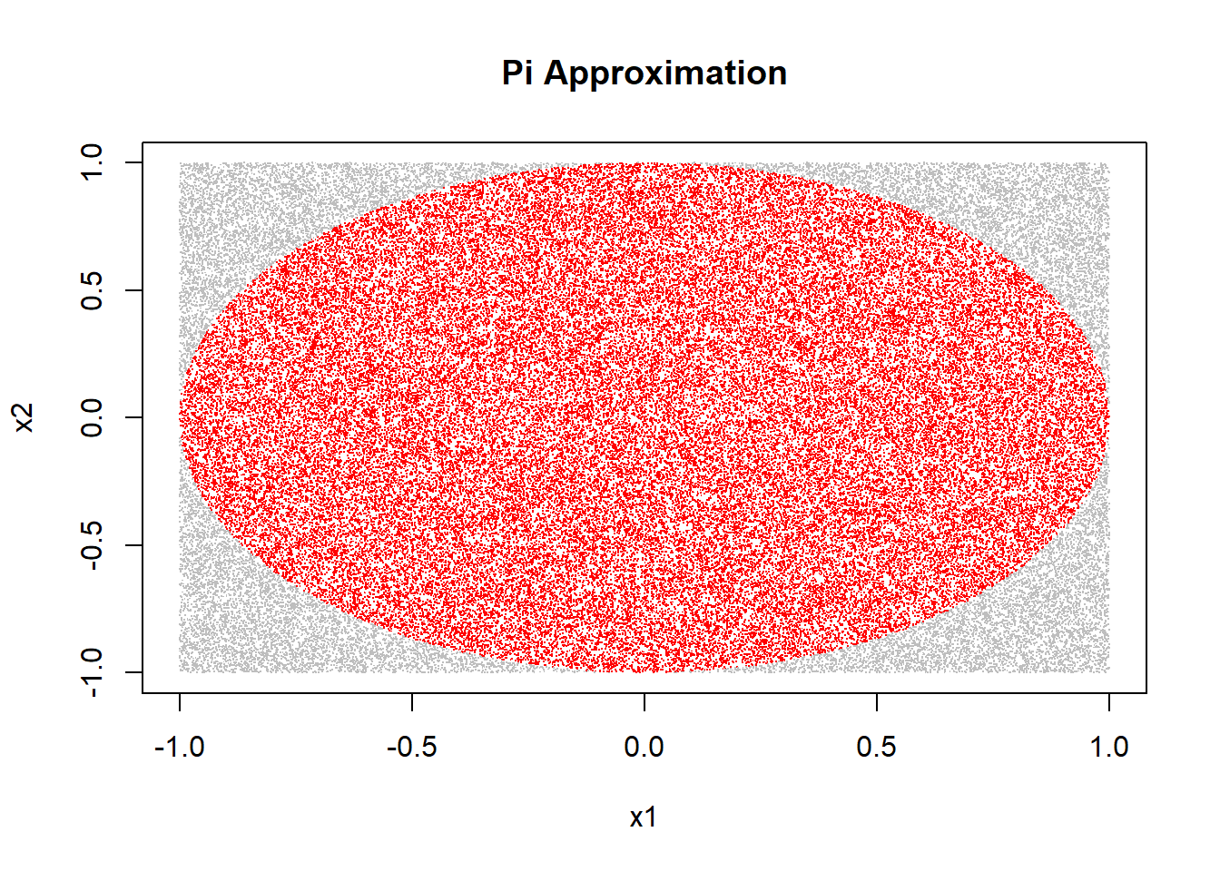
Do not worry if this task was too difficult, it was intended to be an advanced R exercise. In any case, try to understand the solution before reproducing it.
Simulate how often a correlation between two random samples from independent normal distributions is larger than \(.1\). How does this frequency depend on the sample size \(n\)?
Click here to obtain a hint
Sample from a normal distribution through the functionrnorm()
and apply the function cor().
Click here to obtain another hint
If necessary, revisit the chapter on simulations to obtain ways of performing the above operation repeatedly.Click here to see a possible solution
simulate_cor <- function(n) {
    a <- rnorm(n)
    b <- rnorm(n)
    return(cor(a, b))
}

get_cors <- function(n, n_iterations) {
  replicate(n_iterations, simulate_cor(n))
}

# N = 100
n <- 100
n_iterations <- 10000
(sum(get_cors(n,n_iterations)>.1))/n_iterations

# N = 1000
n <- 1000
(sum(get_cors(n,n_iterations)>.1))/n_iterations